GBDT和XGBOOST算法推导和流程详解(PART-1)

写在前面

泰勒公式

泰勒公式是一个用函数在某点的信息描述其附近取值的公式。

基本形式为：

$$f(x) = \sum_{n=0}^n\frac{f^n(x_0)}{n!}(x-x_0)^n \tag{1}$$

以上是泰勒公式的基本定义和基本形式。

泰勒的一阶展开为：

$$\begin{align} &导数定义：\frac{f(x)-f(x_0)}{x-x_0}=f^\prime(x) \to f(x) = f(x_0)+f^\prime(x)(x-x_0) \tag{2}\\ &导数定义另一形式： \frac{f(x+\triangle x)-f(x)}{\triangle x} = f^\prime(x) \to f(x+\triangle x) = f(x)+\triangle xf^\prime(x) \tag{3}\\ &一阶泰勒展开：f(x) = f(x_0)+f^\prime(x)(x-x_0) 或 f(x+\triangle x)=f(x)+\triangle xf^\prime(x) \tag{4} \\ &二阶泰勒展开为：f(x)=f(x_0)+f^\prime(x)(x-x_0)+\frac{1}{2}f^{''}(x)(x-x_0)或\nonumber \\ &f(x+\triangle x) = f(x)+\triangle x f^\prime(x)+ \frac{1}{2} \triangle x^2 f^{''}(x) \tag{5} \end{align}$$

以上可知，导数和泰勒公式是有关系的,因此可以从导数的角度去记忆泰勒公式。

不管是是GBDT还是XGBOOST，只要是base learners到strong learners都会用到这个思想，其迭代的形式可为：

$$\begin{align} 假设：x^t &= x^{t-1}+\triangle x \nonumber \\ 则有：L(x^t) &= L(x^{t-1}+\triangle x)\nonumber \\ &=L(x^{t-1})+\triangle x L^\prime(x^{t-1}) + \frac{1}{2}\triangle xL^{''}(x^{t-1}) \tag{6} \end{align}$$

只不过GBDT用的是一阶，XGBOOST为二阶。

梯度下降法和牛顿法的证明

梯度下降法(Gradient descend)

在机器学习中，最小化损失函数$L(\theta)$，然后求解参数$\theta$，其中比较常用的优化算法是梯度下降法和牛顿法。梯度下降法使用的是损失函数的一阶导数，牛顿不仅用到了一阶导数，而且用到了二阶导数。

$$\begin{align} 迭代公式: \theta^t=\theta^{t-1}+\triangle \theta \nonumber\\ 将L(\theta^t)一阶展开: \nonumber \\ L(\theta^t) = L(\theta^{t-1}+\triangle\theta) \nonumber \\ \simeq L(\theta^{t-1})+\triangle \theta L^\prime(\theta ^{t-1}) \tag{7} \end{align}$$

上式$\theta^{t-1}$可理解成上一轮迭代参数的解，$\theta^t$可理解为本轮参数得到的解，$\triangle \theta$表示本轮迭代参数要变化的量。

$$要使得L(\theta^t)<L(\theta^{t-1}),可取\triangle \theta = -\alpha L^\prime(\theta^{t-1}),则有更新的过程为： \nonumber\\ \theta^t=\theta^{t-1}-\alpha L^\prime(\theta^{t-1}) \tag{8}$$

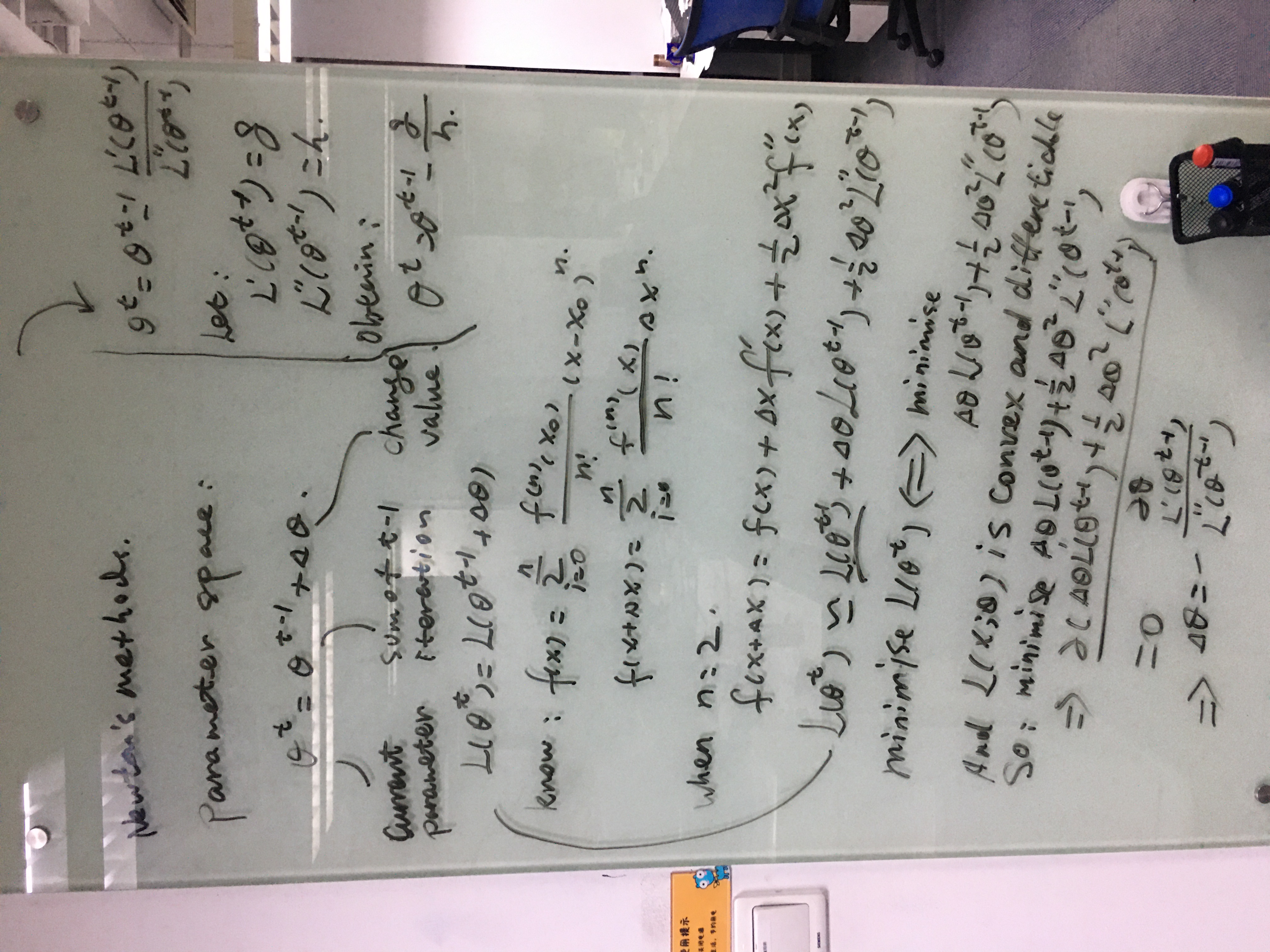
牛顿法（Newtons methods）

$$\begin{align} &迭代公式: \theta^t=\theta^{t-1}+\triangle \theta \nonumber\\ &将L(\theta^t)二阶展开: \nonumber \\ L(\theta^t) &= L(\theta^{t-1}+\triangle\theta) \nonumber \\ &\simeq L(\theta^{t-1})+\triangle \theta L^\prime(\theta ^{t-1})+\frac{1}{2}\triangle \theta^2L^{''}(\theta^{t-1}) \nonumber\\ &= L(\theta^{t-1})+g\triangle \theta +\frac{1}{2}h\triangle \theta^2 \tag{8} \end{align}$$

简化过程，认为参数是标量，要使得$L(\theta^t)$最小，即让$g\triangle \theta +\frac{1}{2}h\triangle \theta^2$极小，则有：

$$\begin{align} &\frac{\partial (g\triangle \theta +\frac{1}{2}h\triangle \theta^2)}{\partial \triangle \theta} = 0 \nonumber \\ &\to \triangle \theta = -\frac{g}{h} \nonumber \\ &\to \theta ^t = \theta^{t-1}-\frac{g}{h} \tag{9} \end{align}$$

即有Newtons methods的迭代公式为$\theta ^t = \theta^{t-1}-H^{-1}G$，$H$为Hessian Matrix.

从参数空间到函数空间

GBDT参数空间

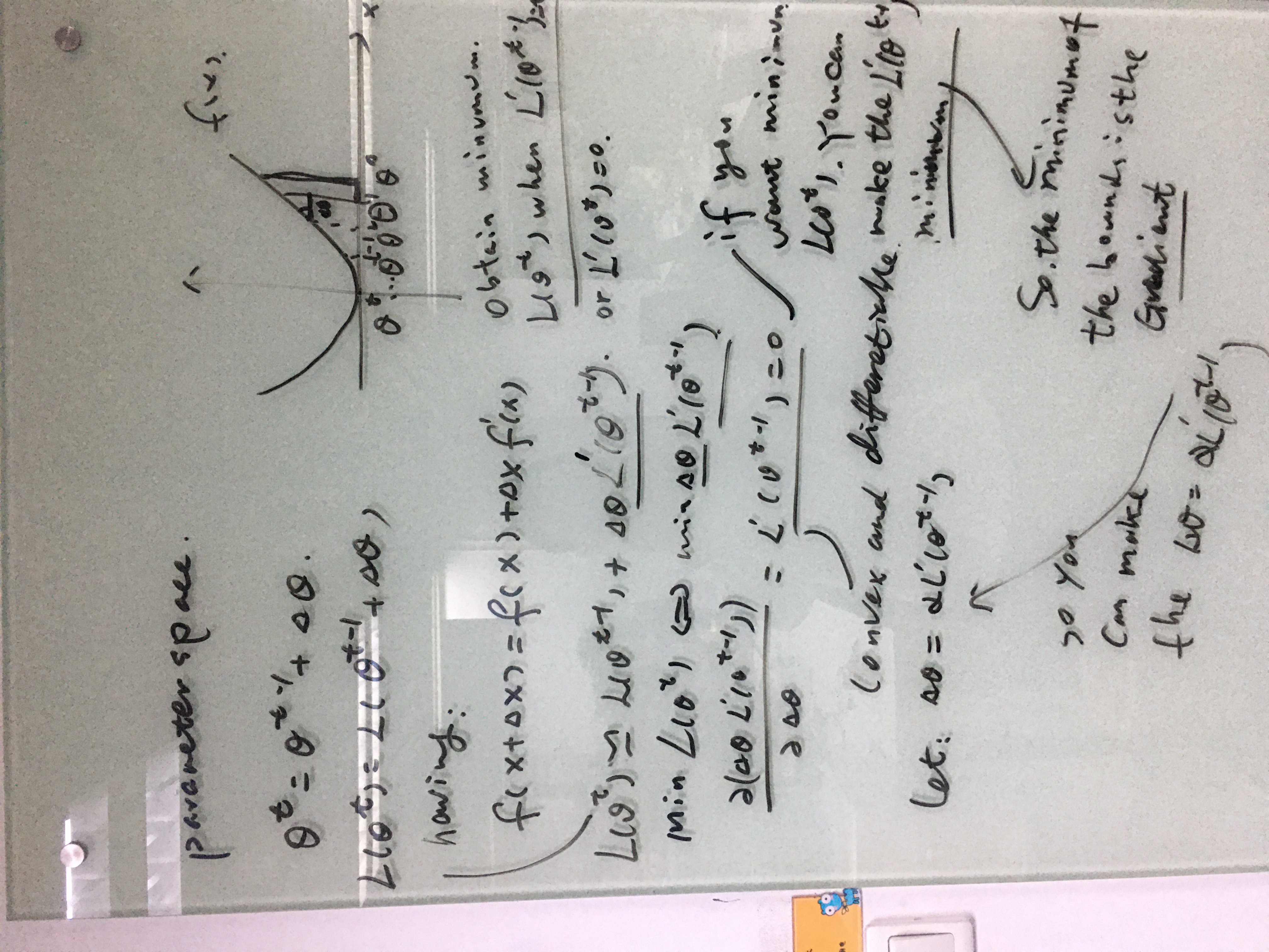
GBDT在参数空间中利用梯度下降法进行更新优化。参数空间：

$$\begin{align} \theta^t &= \theta^{t-1}+\theta_t \nonumber \\ \theta_t& =-\alpha g_t(注意：g_t = L^\prime(\theta^{t-1})) \nonumber\\ \theta &= \sum_{t=0}^T\theta_t \tag{10} \end{align}$$

在参数空间中，最终的参数等于每次迭代的增量的累加和，$\theta_0$为初始值。手推公式如下：

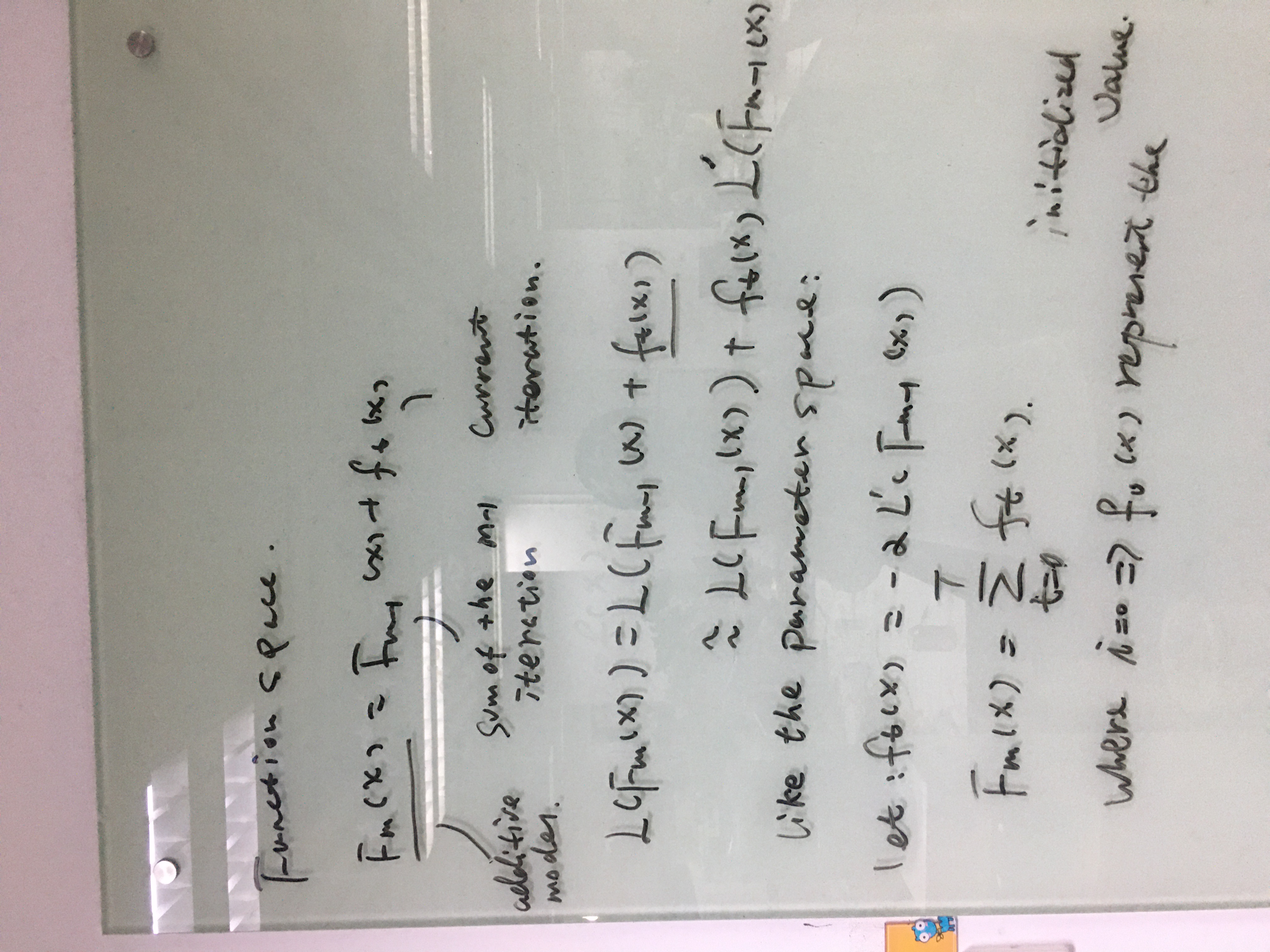
GBDT函数空间

GBDT在函数空间更新的方式基本思想和参数空间很像，即：

$$F^t(x) = F^{(t-1)}(x)+f_t(x) \nonumber\\ f_t(x)=-\alpha g_t(注：g_t = L^\prime(F^{t-1}(x)),如果Loss为均方误差函数：\nonumber\\ \frac{\partial L(F_{m-1(x)})}{\partial F_{m-1}(x)}=y_i-F_{m-1}(x_i) = 残差 \nonumber \\ F(x) = \sum_{t=0}^Tf_t(x)$$

XGBOOST参数空间

XGBOOST参数空间更新优化用到了二阶导数信息。参数空间：

$$\begin{align} \theta^t &= \theta^{t-1}+\theta_t \nonumber \\ \theta_t& =-\frac{g}{h}(注意：g_t = L^\prime(\theta^{t-1}),h_t=L^{''}(\theta^{t-1})) \nonumber\\ \theta &= \sum_{t=0}^T\theta_t \tag{11} \end{align}$$

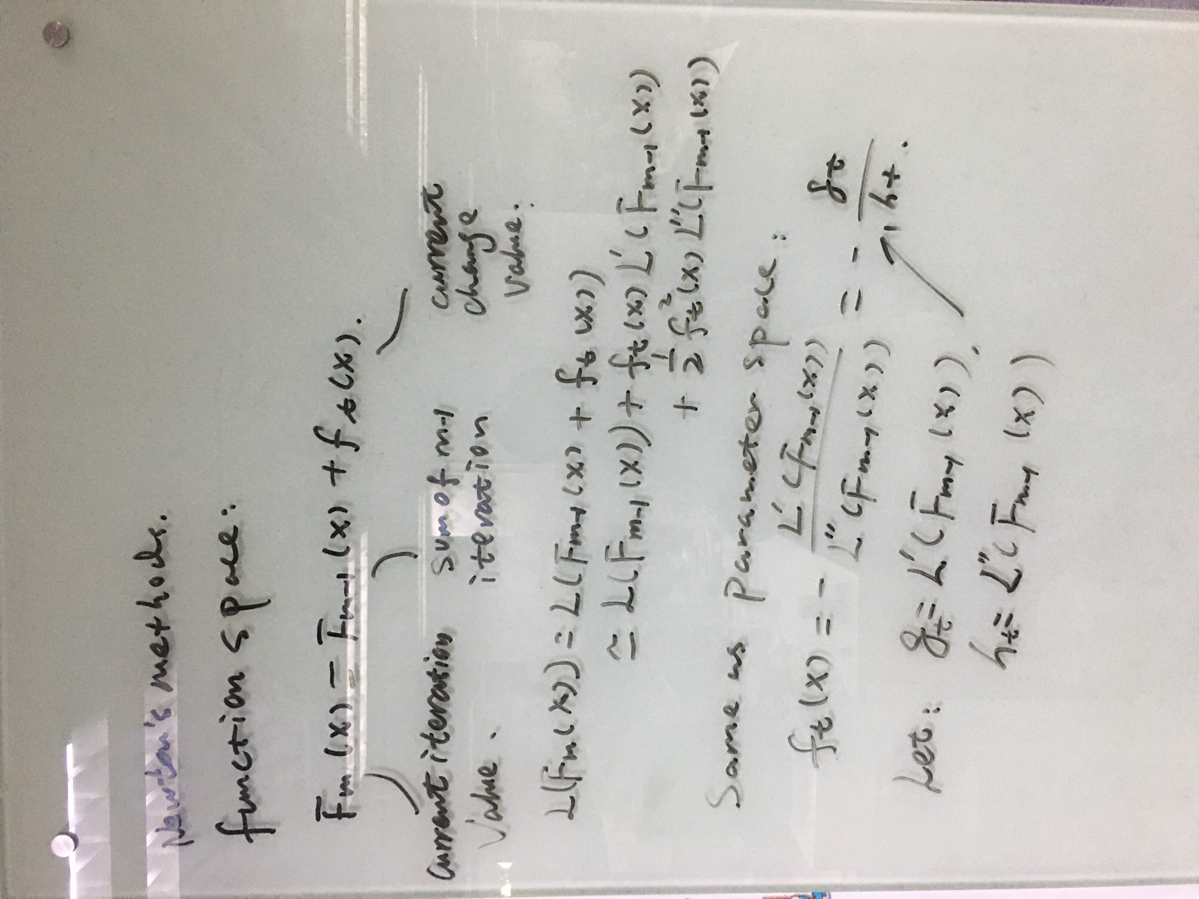
XGBOOST函数空间

在空间中，XGBOOST相比于GBDT来说，使用了二阶信息(牛顿法)。

$$F^t(x) = F^{(t-1)}(x)+f_t(x) \nonumber\\ f_t(x)=-\alpha\frac{ g_t}{h_t}(注：g_t = L(f^{t-1}(x))) \nonumber \\ F(x) = \sum_{t=0}^Tf_t(x) \tag{12}$$

Boosting算法是一种加法模型（addictive model）

$$F(x) = \sum_{t=0}^Tf_t(x) \tag{13}$$

基分类器采用回归树，数模型的优点如下：

1) 不用归一化特征，非线性模型

2）有组合特征作用

3）对缺失值友好，能够很好地处理缺失值

4）异常点对模型结果影响较小（模型非线性）

5）有特征选择作用

GBDT算法原理

算法原理
Friedman于1999年提出的算法，其一般表示方法为：

$$F_m(x;w) = F_{(m-1)}(x)+f_t(x) =\sum_{t=0}^Tf_t(x)\nonumber \tag{14}$$

其中$x$为输入的样本，如果base learners是CART回归树，则有$f_t=h(x;w)=w_{q(x)}$，在这里，回归树的参数为分割点（split point），分割位置（split allocation）和叶子节点的权重。

算法步骤：

第一步：初始化基分类器的初始值为： $f_0=c_0$(很小的数)

第二步：for t in T(Tree number):

（1） 计算$Loss = \sum_{i=1}^nL(y_i,\hat y_i)$对的一阶:

$g_t=\frac{\partial L(y_i,\hat y_i)}{\partial F_{m-1}}|_{\hat y_i = F_{m-1}(x_i)}=(y_i-F_{m-1}(x_i))=residual$ (只有当损失函数均方误差函数时，一

​ 阶导数才是残差)

（2）计算当前迭代树的更新值（一棵新树）： $f_t(x_i)=-\alpha g_t(x_i)$

​ （2-1）利用MMSE方法求得m次迭代的分割点$s$，划分区域$R_1$和$R_2$以及各个区域的平均值作为权重值

​ （2-2）由树的分割点和划分区域的均值得到迭代树：$f_t(x)$

（3）计算$y-F_m(x)$得到残差值，后一棵树在残差值上进行更新

第四步：计算当前迭代后的值：$F_{m}(x) = F_{m-1}(x)+f_t(x)$

if T(迭代的树的棵数) 满足停止条件 or 到达了最优点 :

结束

特征选取和切分方法

对于多个特征而言（m个特征+n个样本），使用贪婪的方式m*n次遍历找到mse最小的分裂点，分裂后，依然在孩子节点上进行划分，遍历的次数为child_left_number*n,右孩子节点要划分的话，计算方式和上面相同。注：每次找splitter都是全部的特征，也就是说一棵树中可能多次复用一个特征。

The features are always randomly permuted at each split. Therefore, the best found split may vary, even with the same training data andmax_features=n_features, if the improvement of the criterion is identical for several splits enumerated during the search of the best split. To obtain a deterministic behaviour during fitting, random_state has to be fixed.

GDBT-SPLIT-Regression

x	1	2	3	4	5	6	7	8	9	10
y	5.56	5.7	5.91	6.4	6.8	7.05	8.9	8.7	9	9.1

某个特征的分割点$s$的判断函数为：

$$\begin{align} split\_function &= \min _{c_1}\sum_{x_i\in R_1}(y_i-c1)+\min_{c_2}\sum_{x_i\in R_2}(y_i-c2) \nonumber\\ s &= \arg\min _s split\_function \nonumber \\ &where \quad R_1 = \{x|x\lt s\},R_2=\{x|x\ge s\} \nonumber\\ &and \quad c_1\frac{1}{N_1}\sum_{i=1}^{N_1}y_i,c_2\frac{1}{N_2}\sum_{i=1}^{N_2}y_i \tag{15} \end{align}$$

按照这个思路，可以通过遍历的方法得到分裂前后的MSE：

s	1.5	2.5	3.5	4.5	5.5	6.5	7.5	8.5	9.5
y	15.72	12.07	8.36	5.78	3.91	1.93	8.01	11.73	15.74

使得分裂函数最小的值就是分裂值，此时最佳分裂点$s=6.5$，且此时的树$f_1(x)=w^{(1)}_{q(x)}$为：

$$T_1(x) =\begin {cases} 6.24(c_1), &x< 6.5 \nonumber\\ 8.91(c_2), &x\ge 6.5 \tag{16} \end {cases}$$

$c_1,c_2$为节点的均值，也就是权重，6.5为特征分割点。
计算残差，然后用回归树拟合残差：

x	1	2	3	4	5	6	7	8	9	10
$r_1$	-0.68	-0.54	-0.33	0.16	0.56	0.81	-0.01	-0.21	0.09	0.14

用$f_1$拟合数据的均方误差为：$L(y,f_1(x))=\sum_{i=1}^{10}(y_i-f_1(x_i))^2 = 1.93$

现在开始拟合第二棵树$f_2(x)$,重复第一棵树的做法，生成第二棵树。

GBDT-SPLIT-Classification

1.不管是分类还是回归，GBDT的特征分裂评价函数都是MSE

2.二分类每次迭代生成一棵树，三分类一次迭代生成3棵树

数据集如下：

样本编号	花萼长度(cm)	花萼宽度(cm)	花瓣长度(cm)	花瓣宽度	花的种类
1	5.1	3.5	1.4	0.2	山鸢尾[1,0,0]
2	4.9	3.0	1.4	0.2	山鸢尾[1,0,0]
3	7.0	3.2	4.7	1.4	杂色鸢尾[0,1,0]
4	6.4	3.2	4.5	1.5	杂色鸢尾[0,1,0]
5	6.3	3.3	6.0	2.5	维吉尼亚鸢尾[0,0,1]
6	5.8	2.7	5.1	1.9	维吉尼亚鸢尾[0,0,1]

三分类的问题，每次训练的目标都是一个one-hot，比如说预测山鸢尾，只有它为0，其他都是0，形成训练样本标签为$y=\{1,1,0,0,0,0\}$.(理解有误)我们用一个三维向量来标志样本的label。[1,0,0] 表示样本属于山鸢尾，[0,1,0] 表示样本属于杂色鸢尾，[0,0,1] 表示属于维吉尼亚鸢尾。

GBDT 的多分类是针对每个类都独立训练一个 CART Tree。所以这里，我们将针对山鸢尾类别训练一个 CART Tree 1，杂色鸢尾训练一个 CART Tree 2 。维吉尼亚鸢尾训练一个CART Tree 3，这三个树相互独立。

先针对第一类进行训练，同样利用mse进行分裂点和分裂特征筛选，选择最小的mse作为分裂特征和分类点。

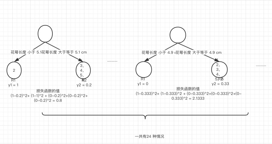
同样，一次迭代的情况下，会同时给出针对第二类和第三类的训练树。

GBDT回归器损失函数
对于回归问题，GBDT采用的损失函数有三个，分别为：MSE(Mean Square Error)， LAD(Least Absolutely Deviation)，Huber(1964,Huber)。

GBDT-MSE-Regression

在处理回归问题的时候，GBDT的损失函数为$MSE=\frac{1}{n}\Sigma_{i=1}^n(y_i-\hat y_i)^2$：

$$\begin{align} L(y_i,\hat y_i) &= \frac{1}{2m}\sum_{i=1}^n (y_i-\hat y_i)^2\nonumber \\ 梯度： &\frac{\partial L(y_i,\hat y_i)}{\partial F_{m-1}(x)}|_{\hat y=F_{m-1}(x)} = \frac{1}{m}(y-F_{m-1}(x)) \tag{16} \end{align}$$

GBDT-LAD-Regression

当损失函数为$LAD=\frac{1}{m}\sum_{i=1}^m\vert y_i - \hat y \vert$:

$$L(y_i,\hat y) = \sum_{i=1}^m\vert y -\hat y \vert \nonumber\\ 梯度:\frac{\partial L(y_i-\hat y)}{\partial \hat y}|_{\hat y = F_{m-1}(x)} = \begin {cases} 1, &y_i-\hat y \ge 0 \nonumber\\ -1, &y_i-\hat y \lt 0 \end {cases} \tag{17}$$

//#huber

The value ofthe transition point δ defines those residual values that are considered to be “outliers,” subject to absolute rather than squared-error loss.

#MSE
class LeastSquaresError(RegressionLossFunction):
    """Loss function for least squares (LS) estimation.
    Terminal regions need not to be updated for least squares. """
    def init_estimator(self):
        return MeanEstimator()

    def __call__(self, y, pred, sample_weight=None):
        if sample_weight is None:
            return np.mean((y - pred.ravel()) ** 2.0)
        else:
            return (1.0 / sample_weight.sum() *
                    np.sum(sample_weight * ((y - pred.ravel()) ** 2.0)))
    
    def negative_gradient(self, y, pred, **kargs):
        return y - pred.ravel()
    
    def update_terminal_regions(self, tree, X, y, residual, y_pred,
                                sample_weight, sample_mask,
                                learning_rate=1.0, k=0):
        """Least squares does not need to update terminal regions.
        But it has to update the predictions.
        """
        # update predictions
        y_pred[:, k] += learning_rate * tree.predict(X).ravel()
    
    def _update_terminal_region(self, tree, terminal_regions, leaf, X, y,
                                residual, pred, sample_weight):
        pass
#LAD
class LeastAbsoluteError(RegressionLossFunction):
    """Loss function for least absolute deviation (LAD) regression. """
    def init_estimator(self):
        return QuantileEstimator(alpha=0.5)

    def __call__(self, y, pred, sample_weight=None):
        if sample_weight is None:
            return np.abs(y - pred.ravel()).mean()
        else:
            return (1.0 / sample_weight.sum() *
                    np.sum(sample_weight * np.abs(y - pred.ravel())))
    
    def negative_gradient(self, y, pred, **kargs):
        """1.0 if y - pred > 0.0 else -1.0"""
        pred = pred.ravel()
        return 2.0 * (y - pred > 0.0) - 1.0
    
    def _update_terminal_region(self, tree, terminal_regions, leaf, X, y,
                                residual, pred, sample_weight):
        """LAD updates terminal regions to median estimates. """
        terminal_region = np.where(terminal_regions == leaf)[0]
        sample_weight = sample_weight.take(terminal_region, axis=0)
        diff = y.take(terminal_region, axis=0) - pred.take(terminal_region, axis=0)
        tree.value[leaf, 0, 0] = _weighted_percentile(diff, sample_weight, percentile=50)
#Huber
class HuberLossFunction(RegressionLossFunction):
    """Huber loss function for robust regression.
    M-Regression proposed in Friedman 2001.
    References
    ----------
    J. Friedman, Greedy Function Approximation: A Gradient Boosting
    Machine, The Annals of Statistics, Vol. 29, No. 5, 2001.
    """

    def __init__(self, n_classes, alpha=0.9):
        super(HuberLossFunction, self).__init__(n_classes)
        self.alpha = alpha
        self.gamma = None
    
    def init_estimator(self):
        return QuantileEstimator(alpha=0.5)
    
    def __call__(self, y, pred, sample_weight=None):
        pred = pred.ravel()
        diff = y - pred
        gamma = self.gamma
        if gamma is None:
            if sample_weight is None:
                gamma = stats.scoreatpercentile(np.abs(diff), self.alpha * 100)
            else:
                gamma = _weighted_percentile(np.abs(diff), sample_weight, self.alpha * 100)
    
        gamma_mask = np.abs(diff) <= gamma
        if sample_weight is None:
            sq_loss = np.sum(0.5 * diff[gamma_mask] ** 2.0)
            lin_loss = np.sum(gamma * (np.abs(diff[~gamma_mask]) - gamma / 2.0))
            loss = (sq_loss + lin_loss) / y.shape[0]
        else:
            sq_loss = np.sum(0.5 * sample_weight[gamma_mask] * diff[gamma_mask] ** 2.0)
            lin_loss = np.sum(gamma * sample_weight[~gamma_mask] *
                              (np.abs(diff[~gamma_mask]) - gamma / 2.0))
            loss = (sq_loss + lin_loss) / sample_weight.sum()
        return loss
    
    def negative_gradient(self, y, pred, sample_weight=None, **kargs):
        pred = pred.ravel()
        diff = y - pred
        if sample_weight is None:
            gamma = stats.scoreatpercentile(np.abs(diff), self.alpha * 100)
        else:
            gamma = _weighted_percentile(np.abs(diff), sample_weight, self.alpha * 100)
        gamma_mask = np.abs(diff) <= gamma
        residual = np.zeros((y.shape[0],), dtype=np.float64)
        residual[gamma_mask] = diff[gamma_mask]
        residual[~gamma_mask] = gamma * np.sign(diff[~gamma_mask])
        self.gamma = gamma
        return residual

GBDT分类问题损失函数

在处理分类问题时，GBDT采用的交叉熵函数，其中对于二分类使用的映射函数为sigmoid函数，多分类使用的soft-max函数。

GBDT-LOSS-CLASSIFIER-BINARY

损失函数：

$$\begin{align} H(p,q) &=-\sum_{j=1}^n \sum_{i=1}^mp_ilogq_i \nonumber \\ & = \sum_{j=1}^n c_0log (1+e^{-F_m(x)})+(1-c_0)(F_m(x)+log(1+e^{-F_m(x)})) \nonumber \\ &\partial Loss(y,\hat y)|_{\hat y = F_{m-1}} = -c_0+\frac{1}{1+e^{-F_m(x)}} = \hat y - y_i \tag{18} \end{align}$$

这个就是GBDT将交叉熵作为损失函数的梯度，当是LR时，由于$F_m = w^Tx$则有梯度为：$(\hat y - y_i)x_i$.

GBDT-LOSS-CLASSIFIER-MULTI

损失函数仍然是交叉熵，但是此时的损失函数形式有些不同：

$$\begin{align} &一个样本：Loss(y_i,\hat y) = -\sum_{j=1}^m y_jlogq_j \tag{19}\\ &只有一个标签为1,其余均为0：Loss(y_i,\hat y) = -log \frac{e^{F^j_m(x_i)}}{\sum_{j^\prime =1}^m e^{F^{j^\prime}_m(x_i)}} \tag{20}\\ 求多分类梯度：&if \quad j = i \to \partial L(y_i,\hat y)|_{\hat y =F_m(x)} = (q_j-1)\nonumber\\ &if \quad j\ne i \to \partial L(y_i,\hat y)|_{\hat y =F_m(x)} = q_j \nonumber\\ &总结多分类梯度计算方式为：g_t|_{F_m(x)} = \hat y_i - y_i \tag{21} \end{align}$$

GBDT梯度计算总结：

//#GBDT梯度计算总结

回归问题：1）损失函数为MSE时：$g_t = (\hat y_i -y_i)$

​ 2）损失函数为LAD：$g_t \in\{1 ,-1\}$，根据预测结果和真实值选择梯度更新

二分类问题： $g_t = \hat y_i -y_i$，其中预测结果$\hat y_i = \frac{1}{1+e^{-F_m(x)}}$

三分类问题：$g_t = \hat y_i -y_i$，其中预测结果$\hat y_i= \frac{e^{F^i_m(x)}}{\sum_{i^\prime}e^{F^{i^\prime}_m(x)}}$

注：后接PART-2(XGBOOST相关内容)